When working with images, as with any kind of signal, we must be aware of resampling issues. A well-known issue that occurs when downsampling images and that has practical implications is aliasing.

In this post I go over how aliasing shows up when using Pytorch’s F.interpolate to downsample images, why it appears, and how we can detect it. I then show how the antialias flag (added in Pytorch 1.11¹) usually solves the issue. If you don’t forget to use it.

Introduction

It is not a new fact that aliasing can have practical implications in neural networks that manipulate image sizes (or any other kind of feature size, actually). A great article by Odena et al.² showed how checkerboard patterns can appear with deconvolution-based upsampling. This is not what we will be talking about today (different from aliasing and we focus on downsampling) but it’s worth reading and the reason actually is quite close to what we will see later.

I knew that aliasing could occur when downsampling images and that it could hinder vision model training and results but it was not until I read “Vision Transformers need Registers”³ (kinda old I know, I have some classics left to be read…) that I realized, thanks to Figure 11 of their paper, how backpropagating a unit gradient through Pytorch’s F.interpolate was a great and intuitive way to visualize the issue and measure how severe it is.

I use this technique and pair it with a quantitative metric (the coefficient of variation of those gradients) to diagnose the aliasing issue in F.interpolate. I then explain how setting the antialias flag to True mitigates the issue, showing when it is the most useful. Interestingly there are still cases where False works better and it has everything to do with how downsampling and antialiasing are implemented.

note

All the code used for making the figures and computing the results in this blog post is available in a detailed notebook you can find here.

The aliasing issue

Introduction to the 1D case

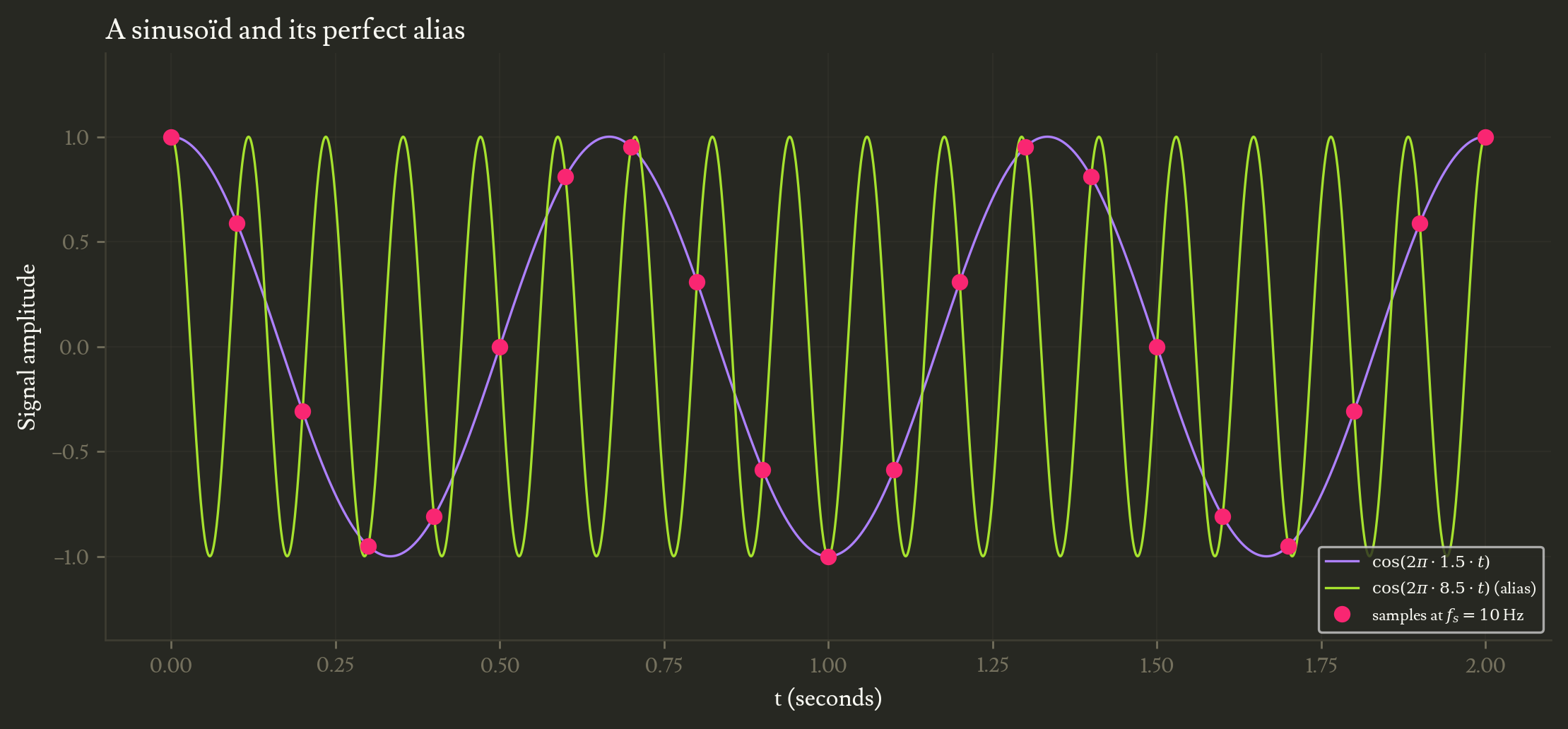
Aliasing does not arise only when downsampling images, it is a well known issue in signal processing that occurs when sampling a signal whose frequency is higher than half the sampling frequency. That half sampling frequency is called the Nyquist frequency⁴.

It is much easier to visualize in 1D first. For instance, let’s consider two perfect sine signals with frequencies $f_1$ and $f_2$, both sampled at a fixed frequency $f_s$. If $f_2 = f_s - f_1$, the samples for both signals match perfectly (see the figure below). Those signals thus cannot be distinguished from each other using samples alone.

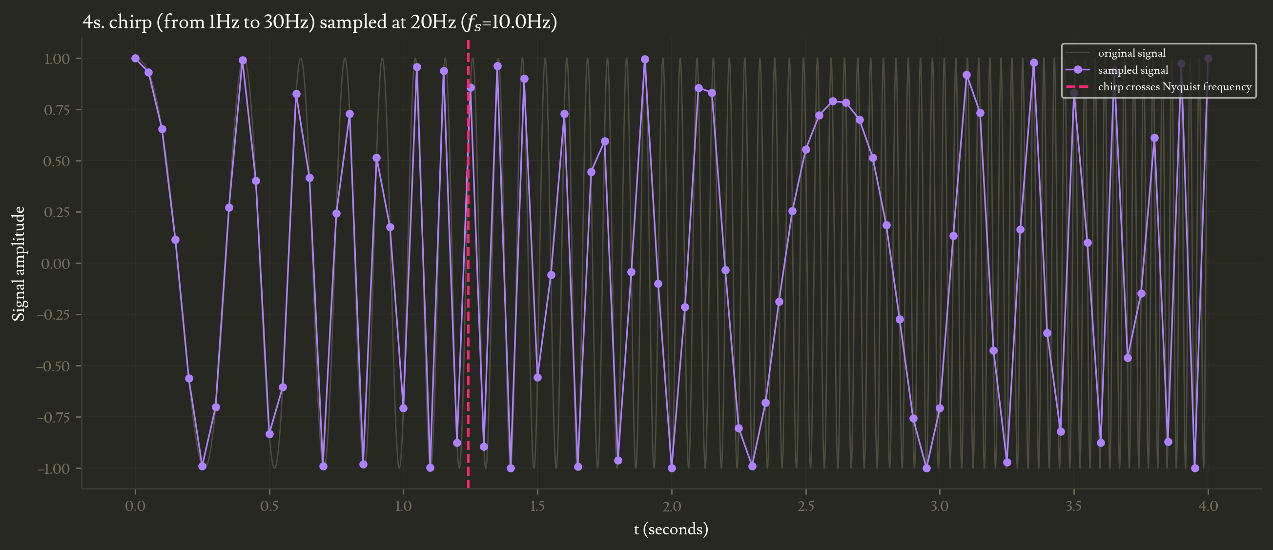
The Nyquist frequency can be easily visualized by sampling a chirp (a sine with continuous frequency increase). See how the signal reconstructed from the samples only (in purple in the figure below) exhibits artifacts once the original signal (in grey) goes past $f_s/2$.

How it shows in 2D images

Images are just 2D signals sampled at whatever resolution we display them. They thus can exhibit similar aliasing issues. This is especially visible when downsampling (resizing to a smaller resolution) images containing high frequency details at a low resolution.

I demonstrate how this looks visually with 3 synthetic examples and 2 real images (from scikit-image⁵).

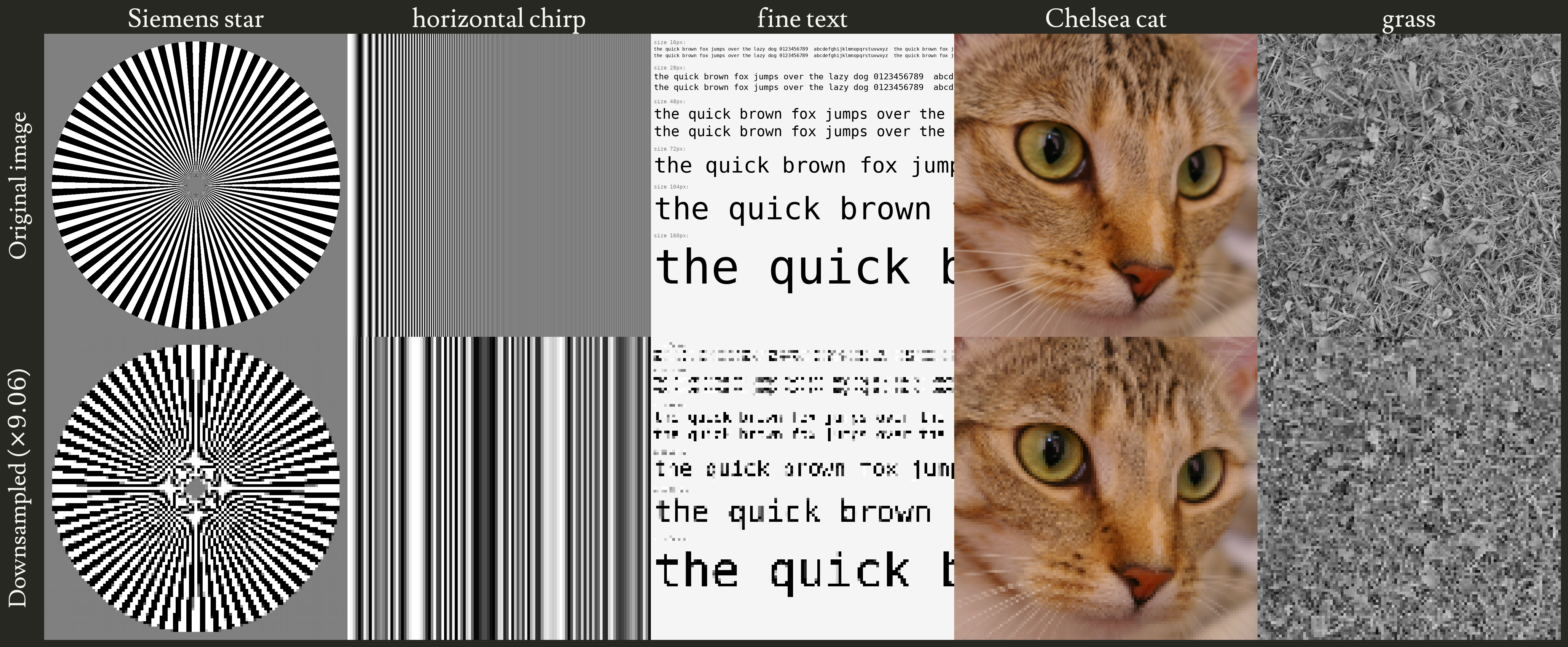
note

You might see aliasing even in the original images if you are reading this on a smaller monitor. If that is the case, open the image in a new tab and view it at 100% scale to ensure the top row is shown at the original resolution.

The Siemens star and the horizontal chirp are the 2D versions of the 1D chirp we took a look at in the previous section. As soon as the frequency goes past the Nyquist frequency (at the center of the star and on the right of the bands) we observe frequency folding artifacts. The Siemens star also suffers from Moiré artifacts⁶. The fine text example shows exactly how downsampling can make OCR pipelines fail or even hallucinate if the input is preprocessed with F.interpolate or other downsampling methods that suffer from aliasing. See how at some lower scale “q” and “b” turn into “o"s for instance, while other strokes disappear. The cat’s whiskers are the prime example of where aliasing shows the most in real images: fine lines that get weirdly jagged when downsampled. Finally, the grass image basically is the worst possible case, having almost only high frequency patterns. It turns into noise after downsampling, losing all semantics.

All those examples demonstrate the same thing: if the original image contains patterns with a frequency higher than the Nyquist frequency for the destination resolution (see the note below), the downsampled image will not only lose those details (this would just be expected data loss) but it will exhibit new patterns with low frequency structure resulting from those high frequencies folding back (exactly how $f_2=f_s-f_1$ was folding onto $f_1$ in the 1D sine example).

note

Defining the Nyquist frequency for images is a bit trickier than with 1D signals. Intuitively, any pattern that has a period smaller than 2 pixels along an axis cannot be faithfully represented and will result in aliasing artifacts. More formally, a destination grid of $N$ samples can represent up to $N/2$ cycles per image width (or height). Any pattern with a higher frequency gets lost and causes folding artifacts.

I found this great and short article that takes this further using 2D Fourier transforms: The Nyquist limit for a two-dimensional detector⁷.

This has direct computer vision consequences because, if overlooked, it can lead to models hallucinating or wasting weight capacity compensating for issues that aren’t even ML-related, but purely mathematical and deterministic. Darcet et al.³ show how the original DINOv2⁸ model suffered from this issue (and how they improved the result with just the simple fix we’ll discuss later).

Measurement of the aliasing issue

For the rest of this post, we will need a better way of detecting aliasing issues and understanding their cause as well as having a proper way of measuring how severe they are for a given operator so we can fairly compare different solutions. Indeed, the previous section showed how aliasing looks on pathological examples but it can be easy to miss (the Chelsea cat for instance only has subtle artifacts).

We will thus define two functions that we will use throughout the post:

• unit gradient map: gives us a visual, qualitative way of explaining aliasing
• coefficient of variation (CV): the single metric we will use to quantitatively measure how severe aliasing can be for a given re-sampling operation

Unit gradient map

This is what lead me to explore and write this blog post. Reading “Vision Transformers need Registers”³, I found it interesting that the authors mention in Appendix A and Figure 11 how they are “propagating unit gradients through a bicubic interpolation” to find out how aliasing was causing some of the artifacts produced by the original DINOv2 model.

The idea is to take advantage of Pytorch’s backpropagation to compute how much each pixel from the original image contributes to the downsampled version.

1. start with a source image filled with ones
2. resample it using the operators of interest (F.interpolate in our case)
3. sum all resulting pixels
4. backpropagate the unit gradient through the operator

note

Note that step 3 is critical because it will allow us to run the backward propagation without biasing the gradient (the derivative of the sum with respect to each pixel is 1). I suggest you take a look at the source notebook, code cell 15, for the actual implementation.

This results in a gradient map: a tensor with the same shape as the source, where each value represents how much the corresponding pixel contributed to the result.

note

After some research I found that this trick seems to have been used for the first time by Luo et al. in 2016 ⁹, where they apply it to a full CNN to visualize its receptive field.

Coefficient of variation (CV)

The unit gradient map gives us a qualitative way of comparing resampling operators but if we want to compare them rigorously we need a quantitative metric. To that end we use the coefficient of variation (I’ll just write CV in the rest of the post).

Where, given a gradient map $g$, $\mu_g$ and $\sigma_g$ respectively denote its mean and its standard deviation.

note

CV is dimensionless: we can thus compare any resampling operator no matter the resulting image size or the method.

Diagnosis

In this section I explore the F.interpolate resampling operator from Pytorch’s functional. I use the two measures defined above to check how bad aliasing can get and find the critical cases.

Downsampling modes and ratios

Taking a look at the F.interpolate documentation, there are two main parameters that affect the result:

• mode: resampling algorithm
• scale_factor: we derive this from the source and destination resolutions to resize the image to the desired dimension

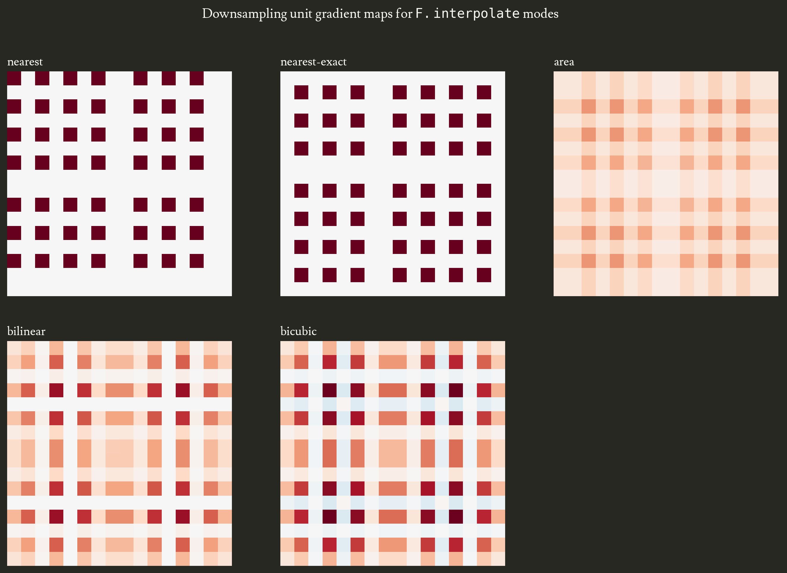
Let’s start by exploring how modes affect the unit gradient map (and take a first look at what we defined above actually looks like!).

note

nearest and nearest-exact are almost the same: nearest-exact was added to fix known coordinate issues in nearest, kept for backward compatibility¹⁰.

The nearest mode looks the worst and the reason is simple: some pixels contribute fully to the result while others are purely ignored. Bilinear and bicubic look very similar. Their pattern is identical, only the value scale changes: the bicubic, due to its odd exponent, goes to negative values and in general shows more “contrast”, worsening the disparity in its unit gradient maps. Area downsampling basically is box filtering, which has the side effect of resulting in a slightly blurry image but it helps a lot when it comes to aliasing. It basically is the best downsampling mode when you need to avoid aliasing by default.

Let’s check the actual CV for those modes. I compute CV in three scenarios:

• $16 \times 16 \rightarrow 7 \times 7$: great small example with a non-integer downsampling ratio. It’s also the kind of ratio used by DINOv2⁸’s positional-embedding interpolation when running the model on smaller-than-default inputs (source)
• $16 \times 16 \rightarrow 8 \times 8$: same source size but a common integer $2\times$ ratio
• $1024 \times 1024 \rightarrow 113 \times 113$: matches the synthetic and natural-image example used earlier in the post. The $\approx 9\times$ ratio is aggressive and non-integer, stacking both pathologies in one scenario.

As expected, nearest and its exact variant show the worst CV scores for all three scenarios. Note that area mode does beat bilinear and bicubic and sustains a low CV in all scenarios. The difference between the bilinear and bicubic modes is mainly explained by the negative contribution of some pixels we mentioned earlier with the cubic kernel.

When we only consider some fixed resizing ratios, it’s easy to miss interesting patterns, I thus plot the CV for a range of those ratios.

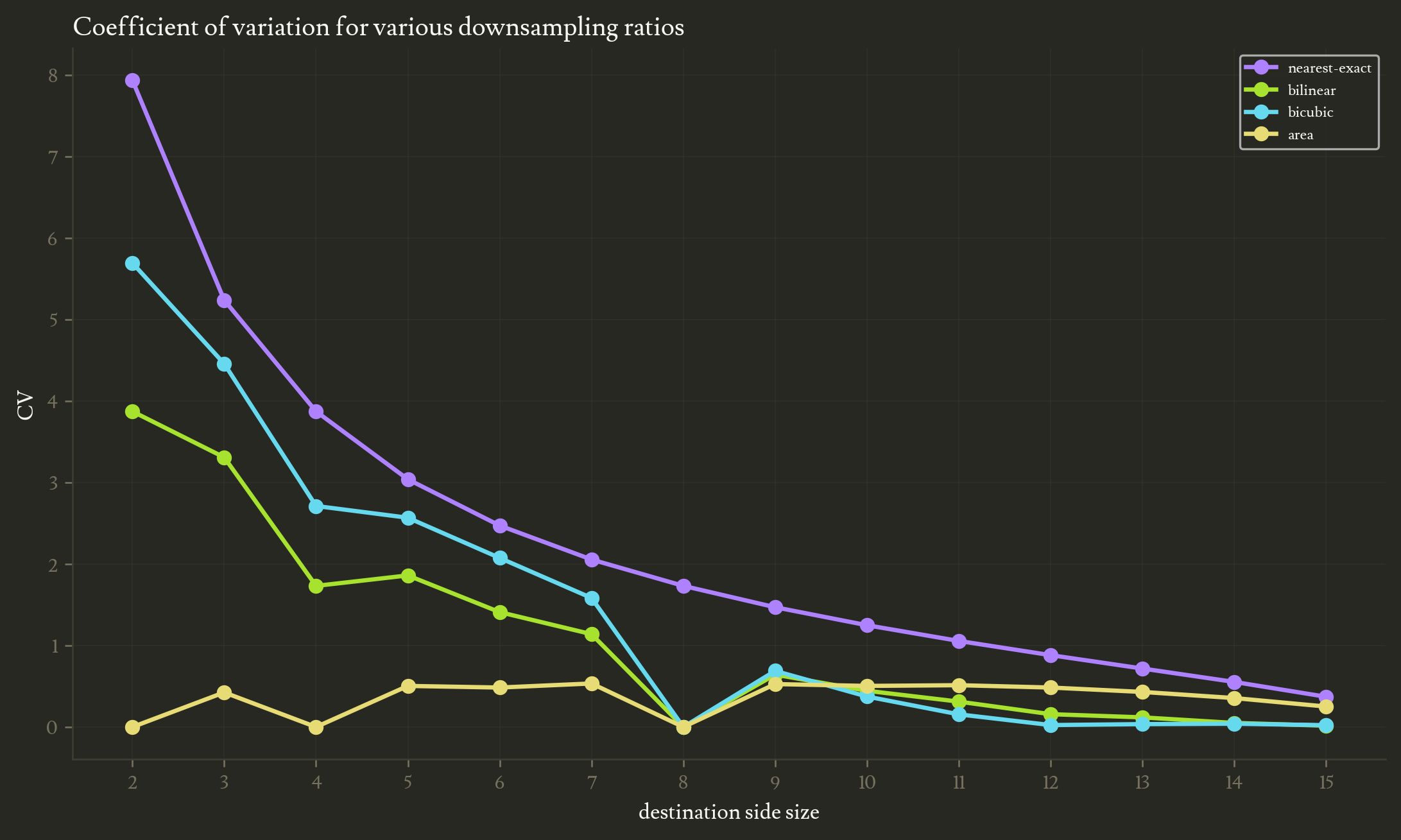
As we expect the aliasing issue gets increasingly strong as we lower the destination resolution.

note

The CV has a closed form for the nearest mode. In downsampling each source pixel gets gradient $0$ or $1$ (either some output picks it or none does), and exactly $\text{dst}^2$ source pixels are picked, so the Bernoulli CV gives

$$\mathrm{CV}_{\text{nearest}} = \sqrt{\left(\frac{\text{src}}{\text{dst}}\right)^2 - 1}$$

The most notable observation to be done is how all modes except nearest dip on integer downsampling ratios ($16/8$, $16/4$, $16/2$). This is because at those ratios, the receptive fields of those downsampling modes can cleanly be repeated and cleanly tile the source image without overlapping each other. Hence, each pixel from the source image has the exact same contribution to the downsampled destination.

Observe how area usually is better than bilinear and bicubic for higher downsampling ratios. I could stop there and tell you that you should use the area mode when downsampling, and while that is partially true, this mode has some visual issues (it just is a box filter so results are a bit blurry for instance). Moreover, the fix I’ll discuss in the Solution section is not applicable to the area mode. For the rest of this post I’ll thus focus on the bicubic mode because it is the default mode in most functions/libraries and it is the most commonly used one.

Side note about upsampling

In the upsampling case (destination size higher than the source), every frequency in the source lies below the destination’s Nyquist frequency, so nothing folds and no aliasing arises.

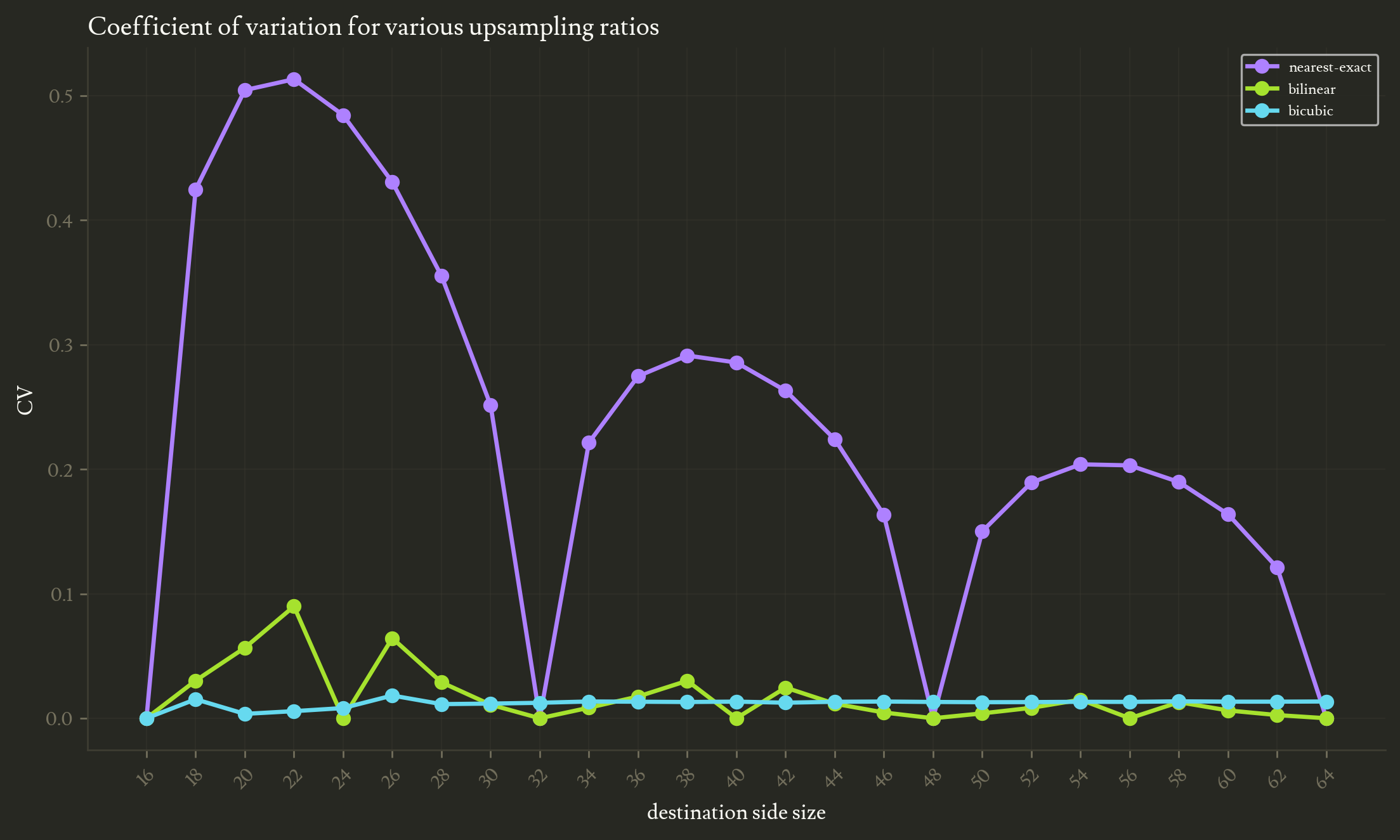
The scale of CV here is way lower than in the downsampling sweep.

It’s still worth noting that nearest-exact shows non-negligible CV at non-integer upsampling ratios. This isn’t due to aliasing though, it is because between integer ratios, some source pixels are used more than others in the result. This mode replicates exactly one source pixel for each destination pixel, and since the destination size isn’t an integer multiple of the source size, some source pixels necessarily get replicated more than others.

Solution

Easy: set antialias=True

Pytorch 1.11 release introduced an antialias flag to F.interpolate and while the exact way it works depends on the mode, the core idea is to make the downsampling algorithm scale-aware¹. Indeed, while the regular bicubic mode uses a fixed-size kernel of $4 \times 4$ pixels, enabling antialias widens it to $4/R$ pixels per axis where $R = \frac{\text{dest}}{\text{src}}$ is the resampling ratio. The reason it helps avoid aliasing is that stretching the kernel by $1/R$ compresses its frequency response by $R$, which lowers the kernel’s cutoff from the source Nyquist down to the destination Nyquist.

Let’s compare the unit gradient map when antialias=True with the one we previously took a look at.

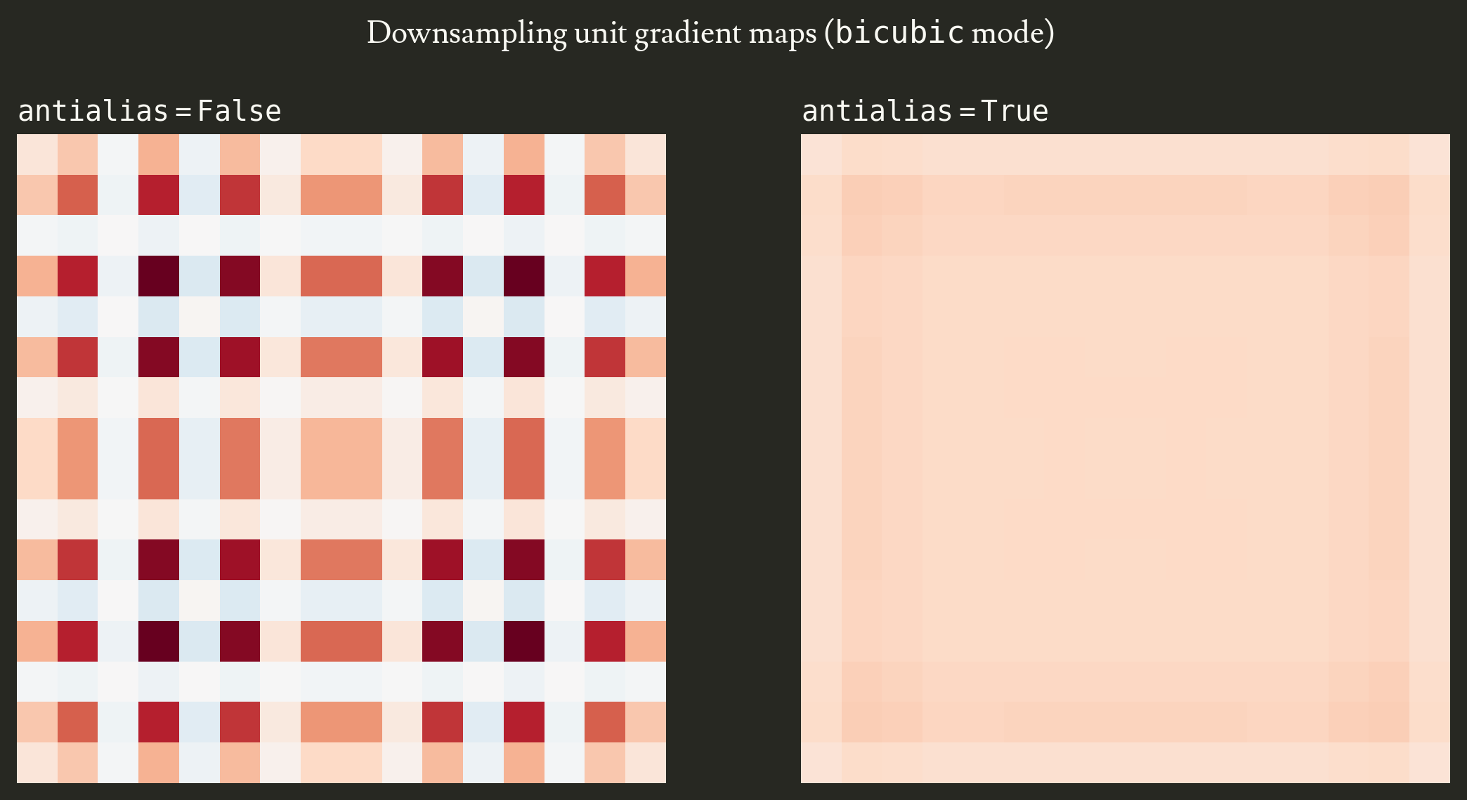
As I previously showed, without antialiasing the unit gradient map is highly irregular with a structured checkerboard of pixels that are either overused or underused to produce the destination image, yielding a high CV of 1.58. With antialiasing (on the right), the unit gradient map becomes almost uniform and the CV drops to 0.11.

note

There is a slight edge artifact that appears when using antialiasing, it is the only reason the CV isn’t zero. It is due to the widened kernel being clipped at the source image’s edges. This implies that source’s edge pixels contribute less to the destination.

The same effect shows on the natural-image examples from earlier.

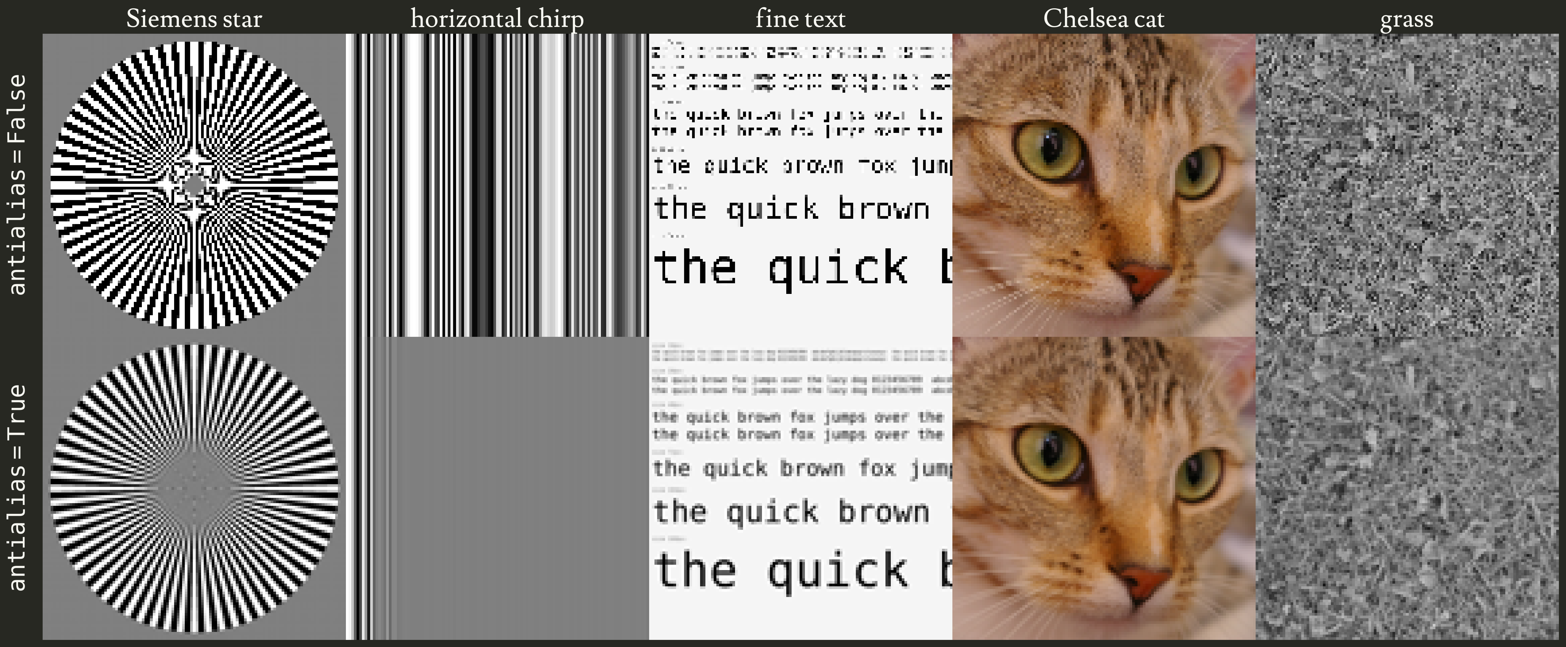
Moiré disappears from the Siemens star center, the chirp’s high-frequency bands stop folding, fine text becomes readable, the cat’s whiskers stay continuous, and the grass texture no longer collapses into noise… at the cost of the destination images looking slightly blurry. Details from the source image are now lost without creating new details from frequency folding.

Sweeping CV across destination sizes confirms this quantitatively.

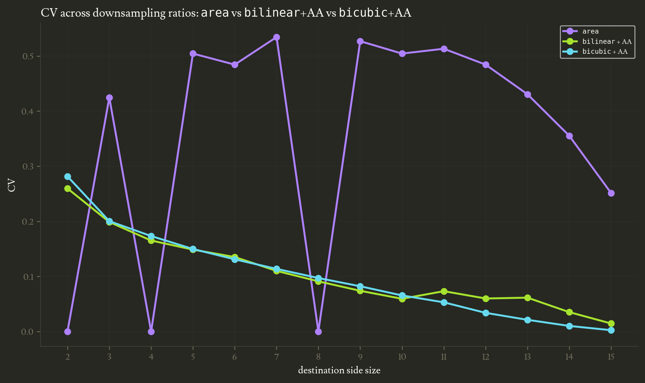
Antialiased bilinear and bicubic stay low and nearly identical across all ratios, while area oscillates between zero (at integer ratios, where its box filter tiles cleanly) and the 0.5 region (at non-integer ratios). Antialiased bicubic now dominates area at every non-integer ratio.

The CV landscape

Until now I only explored specific downsampling ratios (mostly from $16 \times 16$ to $7 \times 7$ for reasons mentioned above). In this section I’ll take a more exhaustive approach by plotting a heatmap of the CV depending on the source and the destination sizes. Since I only consider downsampling, the heatmap is triangular.

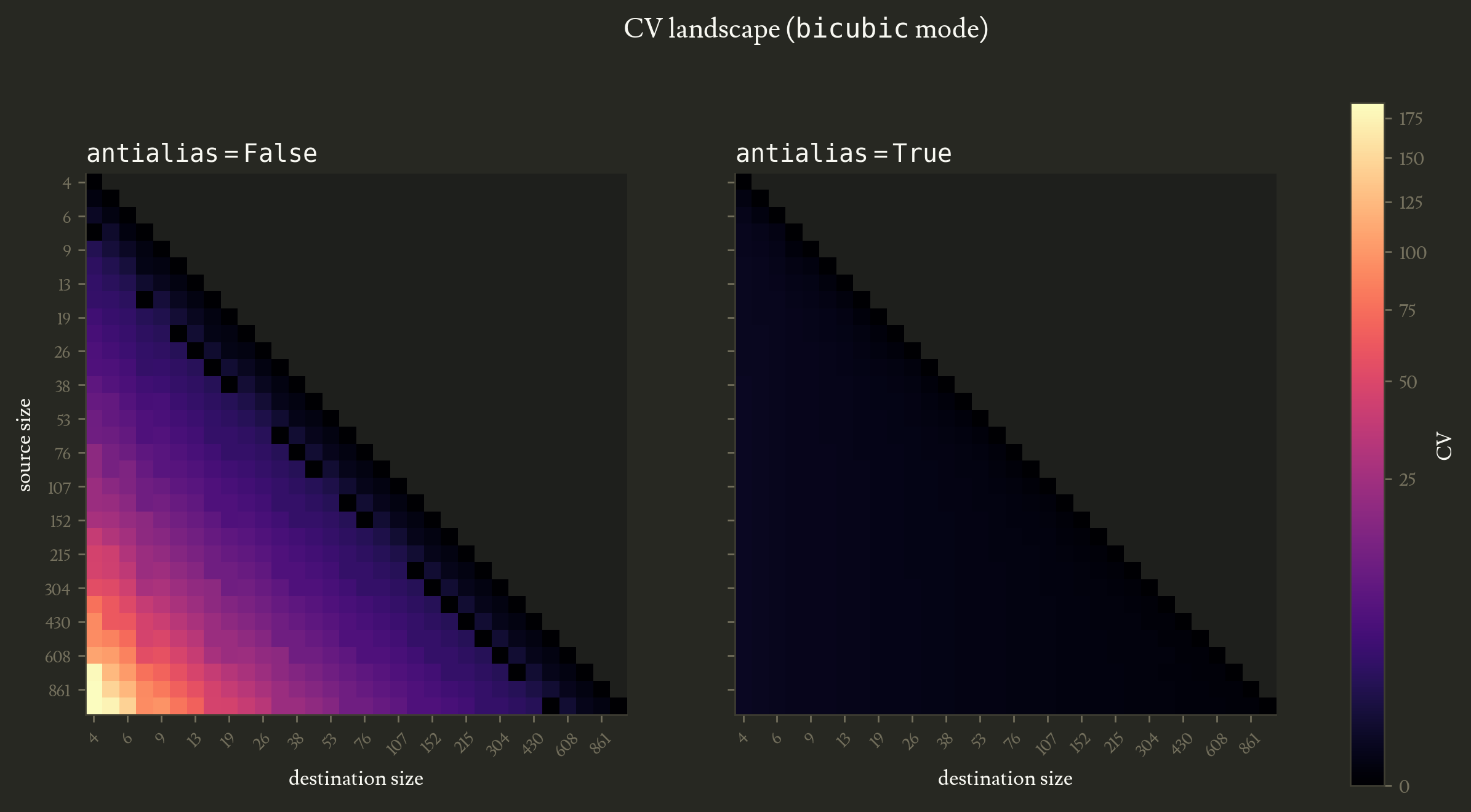
important

I used a power-law color scale to compress the high-CV end so variation in the antialiased plot stays visible while both plots share the same scale. The CV with antialiasing really is much lower than without.

The clearest observation is that antialiasing greatly reduces CV in most cases. Note the black diagonal in the left heatmap though, it corresponds to a perfect downsampling by a factor of 2, that, as I previously mentioned, has no aliasing issue. The trend we saw in the previous section, CV growing as the downsampling ratio gets more extreme, is confirmed in the general case.

When NOT to antialias

Although the previous sections suggest that antialias should be set to True whenever downsampling, there are two main cases where I would suggest not using antialiasing.

The first is when the downsampling ratio is known to be exactly 2. As I previously mentioned, in that situation the no-antialias bicubic shows a clean CV of 0 while using antialiasing will yield a slightly positive CV due to the edge artifacts and, in general, lose slightly more image details than without antialiasing.

Another reason to avoid antialiasing is when you really really don’t want to increase your compute time. Indeed, since antialias=True widens the resampling kernel, the operation needs to process more source pixels, which increases the processing time.

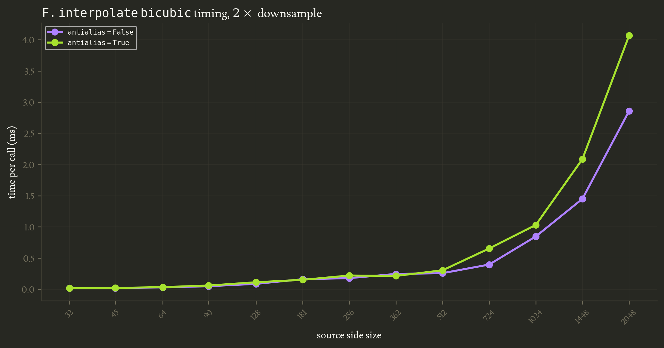
The plot above (each point is an average of 1000 runs) shows how the computation time for downsampling:

• increases as the source size increases
• is slightly higher when antialiasing

But honestly the computing overhead of antialiasing is so negligible that I would not care unless I was processing billions of images of very high resolution.

Conclusion

Using the unit gradient map trick and computing the coefficient of variation on these maps we can easily track how image resampling operators act on the input pixels. It surfaces where the aliasing happens when downsampling and how severe it is.

The practical conclusion is clear: unless you are downsampling by a known integer ratio, the bicubic mode of F.interpolate with antialias set to True is the cleanest option for avoiding aliasing.

While the fix, setting that antialias flag introduced by Pytorch 1.11, is easy, it is very common to forget it. Coming back to the introduction, Darcet et al.³ found out that the DINOv2⁸ suffered from aliasing issues in the positional embeddings.

I only considered F.interpolate in this blog post but it’s far from the only downsampling operator used in vision models. The figure below shows how Conv2D and MaxPool2D also have aliasing issues. I found that Odena et al.² studied the visual artifacts caused by transposed convolution but while it is an interesting read it only is adjacent to the aliasing issue in downsampling.

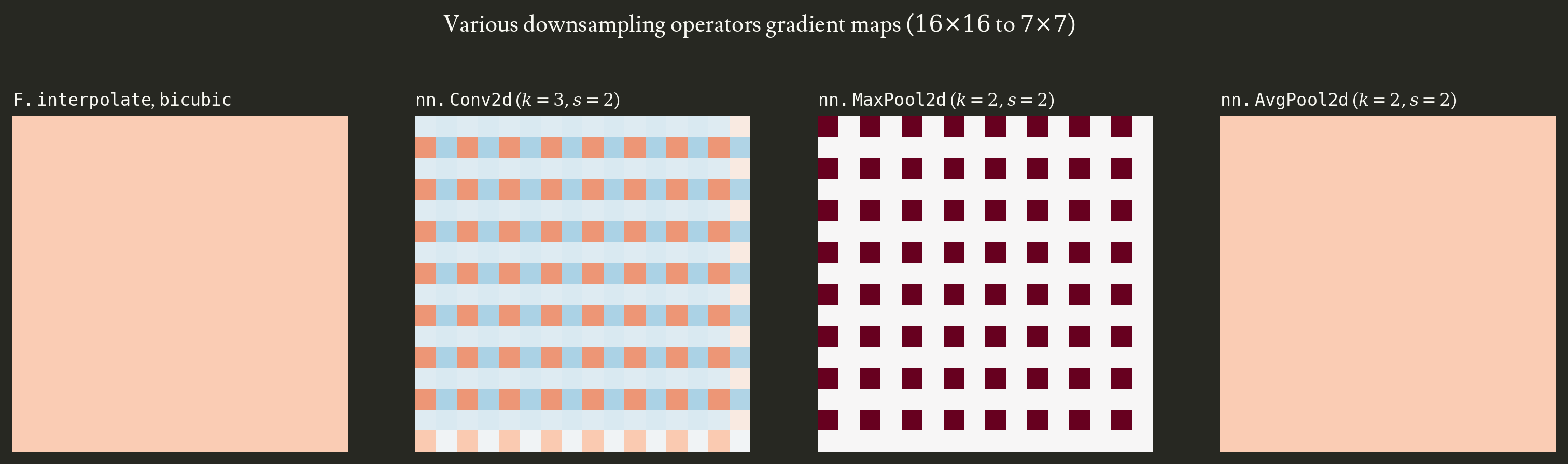
All figures and computations are reproducible from the source notebook.

References

PyTorch contributors. (2021). Add
antialiasflag toF.interpolate(Pull request #68819). GitHub. https://github.com/pytorch/pytorch/pull/68819 ↩︎ ↩︎Odena, A., Dumoulin, V., & Olah, C. (2016). Deconvolution and Checkerboard Artifacts. Distill, 1(10), e3. https://doi.org/10.23915/distill.00003 ↩︎ ↩︎
Darcet, T., Oquab, M., Mairal, J., & Bojanowski, P. (2024). Vision Transformers Need Registers (arXiv:2309.16588). arXiv. https://doi.org/10.48550/arXiv.2309.16588 ↩︎ ↩︎ ↩︎ ↩︎
Nyquist frequency. (n.d.). In Wikipedia. Retrieved May 20, 2026, from https://en.wikipedia.org/wiki/Nyquist_frequency ↩︎
van der Walt, S., Schönberger, J. L., Nunez-Iglesias, J., Boulogne, F., Warner, J. D., Yager, N., Gouillart, E., Yu, T., & the scikit-image contributors. (2014). scikit-image: image processing in Python. PeerJ, 2, e453. https://doi.org/10.7717/peerj.453 ↩︎
Moiré pattern. (n.d.). In Wikipedia. Retrieved May 22, 2026, from https://en.wikipedia.org/wiki/Moir%C3%A9_pattern ↩︎
Sutin, B. M. (2025, January 11). The Nyquist limit for a two-dimensional detector. Skewray Research. https://www.skewray.com/articles/the-nyquist-limit-for-a-two-dimensional-detector ↩︎
Oquab, M., Darcet, T., Moutakanni, T., Vo, H., Szafraniec, M., Khalidov, V., Fernandez, P., Haziza, D., Massa, F., El-Nouby, A., Assran, M., Ballas, N., Galuba, W., Howes, R., Huang, P.-Y., Li, S.-W., Misra, I., Rakotosaona, M., Mainberger, F., Jegou, H., Labatut, P., Joulin, A., & Bojanowski, P. (2023). DINOv2: Learning Robust Visual Features without Supervision (arXiv:2304.07193). arXiv. https://doi.org/10.48550/arXiv.2304.07193 ↩︎ ↩︎ ↩︎
Luo, W., Li, Y., Urtasun, R., & Zemel, R. (2016). Understanding the effective receptive field in deep convolutional neural networks. In Advances in Neural Information Processing Systems 29 (NIPS 2016). https://proceedings.neurips.cc/paper/2016/hash/c8067ad1937f728f51288b3eb986afaa-Abstract.html ↩︎
torch.nn.functional.interpolate. (n.d.). In PyTorch 2.12 documentation. Retrieved May 26, 2026, from https://docs.pytorch.org/docs/2.12/generated/torch.nn.functional.interpolate.html ↩︎