Bad Apple but it's GPT-2 XL Attention Maps

“Can it display Bad Apple?” is the “Can it run Doom?” of displays: since the 2010s, people have been trying to display the Bad Apple music video on anything that can show grayscale images, ranging from Desmos graphing calculator to Tesla coils and lasers¹.

I wanted to adapt this meme to machine learning and thought of various ways of doing it, but using an image generation model for that seemed too straightforward so I wanted something sillier. What if we used an LLM (that never saw any image) and tried to bend it so that its attention maps display the video frames?

What are attention maps?

Transformers such as the GPT-2 XL LLM process text using a mechanism called attention: for each token in the input, the model computes a score against every other token to decide how much information to pull from it. These scores are stored in a matrix called “attention map”.

If we feed the model a sequence of 256 tokens, each token attends to all 256 tokens, giving us a 256×256 matrix of attention weights. That’s a 256×256 grid of values and a 256×256 grid of values is just… an image.

That’s the core idea: the attention map is our display. We tweak the model inputs until the attention maps look like our target frames.

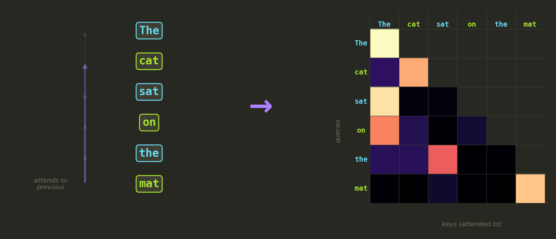Each cell shows how much a token (row) attends to another token (column). The black triangle is the causal mask.

Why GPT-2 XL?

Regarding the model choice, I was looking for a small model (for efficiency and simplicity) that would easily expose the attention maps. Thought about Llama, Mistral or Qwen but recent models are more complex than needed so I landed on GPT-2 (chose the XL variant to give the optimizer more degrees of freedom but the small model could have worked too).

Still, GPT-2 XL has some nice properties for our project:

• it uses MHA where every head has its own set of Q/K/V values
• we have full access to the raw attention weights (you’ll see why it’s important in the following sections), this is not the case with many newer models that use GQA or FlashAttention
• it’s tiny, fits in 3.2GB in fp16
• it has very few moving parts, especially since we only use the Q and K slices and do the matmul ourselves (see the following sections)
• and, I’ll admit it, GPT-2 is a well known name that makes for a great post!

Method

The core idea

I freeze the entire GPT-2 XL model and only optimize the input. Normally you’d feed the model actual text tokens, but here I bypass the token embedding table entirely and optimize a raw embedding tensor directly, a 256×1600 matrix of floating point values, one row per token position.

Note that instead of running the full forward pass, I only do the following:

where $X$ is the learnable 256×1600 input, $W_{\text{pos}}$ are the frozen position embeddings, and $W_Q$, $W_K$ are the frozen Q/K weight matrices of a single attention head (note that I don’t even compute the V values). $A$ is the resulting 256×256 matrix of raw attention scores (the “display”).

Each frame of Bad Apple gets its own independently optimized embedding.

The naive approach (and why it doesn’t work)

I naively tried to use all the attention maps of the GPT-2 XL model to render the whole video in very few passes: GPT-2 XL has 25 attention heads per layer, each producing its own 256×256 attention map. Optimize a single shared input, get 25 frames at once. With 3286 frames, that’s only ~130 runs which would have been efficient.

But this fails badly, mainly due to two reasons:

• each head’s Q and K projections slice 64 dimensions out of the shared 1600-dimensional input. For 25 independent attention patterns, the heads collectively need 25 × 64 × 2 = 3200 degrees of freedom. The input only has 1600. The heads fight over the same numbers and every frame comes out as a blurry compromise.
• the attention weights come out of a softmax, and backpropagating through it squashes gradients to near-zero. The optimizer has a signal, but it’s ~250× too faint to make progress.

Things I tried that didn’t help:

• more optimization steps (loss flatlines after ~200)
• LBFGS instead of Adam (converges to the same plateau)
• cosine annealing with warm restarts (marginal improvement)
• gradient clipping (no effect)
• using multiple layers instead of one (same overconstrained problem, just spread across layers)

After all this, loss plateaued at 5.85 and refused to budge.

What actually worked

Instead of squeezing 25 frames out of one input, give each frame its own input and target a single attention head. This requires me to run a new forward pass for each frame and is a bit less elegant but it allows the optimizer to have much more freedom and makes it easier for the training process to converge.

Single head targeting

I pick head 0 of layer 0 and give each frame its own independently optimized 256×1600 embedding. The overconstrained problem just disappears: each head only uses $64 + 64 = 128$ dimensions for its Q and K projections, while the input has 1600. Going from fighting over shared capacity to having more degrees of freedom than needed. Loss dropped from 5.85 to 0.29, a ×19 improvement.

Note that I batch 64 frames on GPU at once (each with its own independent input) to keep things efficient.

Logit-space MSE loss

This is the single biggest improvement after single-head mode. Computing MSE on the attention weights themselves (post-softmax) gives gradients on the order of $10^{-5}$, way too faint. Instead, I skip the softmax entirely and compute the loss directly on the raw attention scores $A$ (pre-softmax logits). For each target frame, I convert the target attention distribution to desired logits:

The row-wise centering is needed because softmax is shift-invariant: $\text{softmax}(\mathbf{x}) = \text{softmax}(\mathbf{x} + c)$ for any constant $c$. Without centering, the optimizer would waste effort adjusting the overall scale of logits without changing the attention pattern. The loss is then just MSE between the centered predicted logits and these desired logits, computed within the causal mask:

where $\mathcal{M}$ is the set of positions in the lower triangle (causal mask). This gave gradients around $10^{-2}$, roughly 250× stronger than before.

Multi-seed exploration

The attention landscape is non-convex and Adam can get stuck in bad local minima. To deal with this, I start from 3 random initializations and run each for 375 steps (explore phase), keep whichever seed produced the lowest loss, then continue optimizing that one for 1125 more steps (refine phase). That’s 1500 effective optimization steps per frame. I also use a cosine annealing scheduler with warm restarts to periodically reset the learning rate and escape plateaus.

This is a well-known technique called multi-start optimization²: run the same optimizer from different random starting points and keep the best result. It’s one of the easiest ways to help the optimizer converge on non-convex or complex loss landscapes.

Post-processing

The optimization gives raw attention logits, but turning those into a good-looking frame takes some work. Raw attention weights after softmax are all very close to each other (they form a probability distribution, most values hover near $1/n$), so I apply:

1. per-row z-score normalization to reveal relative attention patterns instead of absolute values
2. percentile clipping (1st–99th) to remove extreme outliers
3. gaussian blur ($\sigma=1.5$) to smooth out horizontal streak artifacts from the row-wise normalization
4. magma colormap for… the “attention map” aesthetic and because it looks cool :D

Note that this post processing is done after the optimization so it doesn’t play in the learning process. It’s purely visual processing to help us visualize the results.

Results

Final results

The whole pipeline runs on 3286 frames (Bad Apple at 15fps, 256×256 grayscale). On an RTX 5070 Ti, the full optimization takes about 12 minutes, roughly 0.23 seconds per frame, batching 64 frames at a time on GPU. Peak VRAM sits at around 4.5 GB.

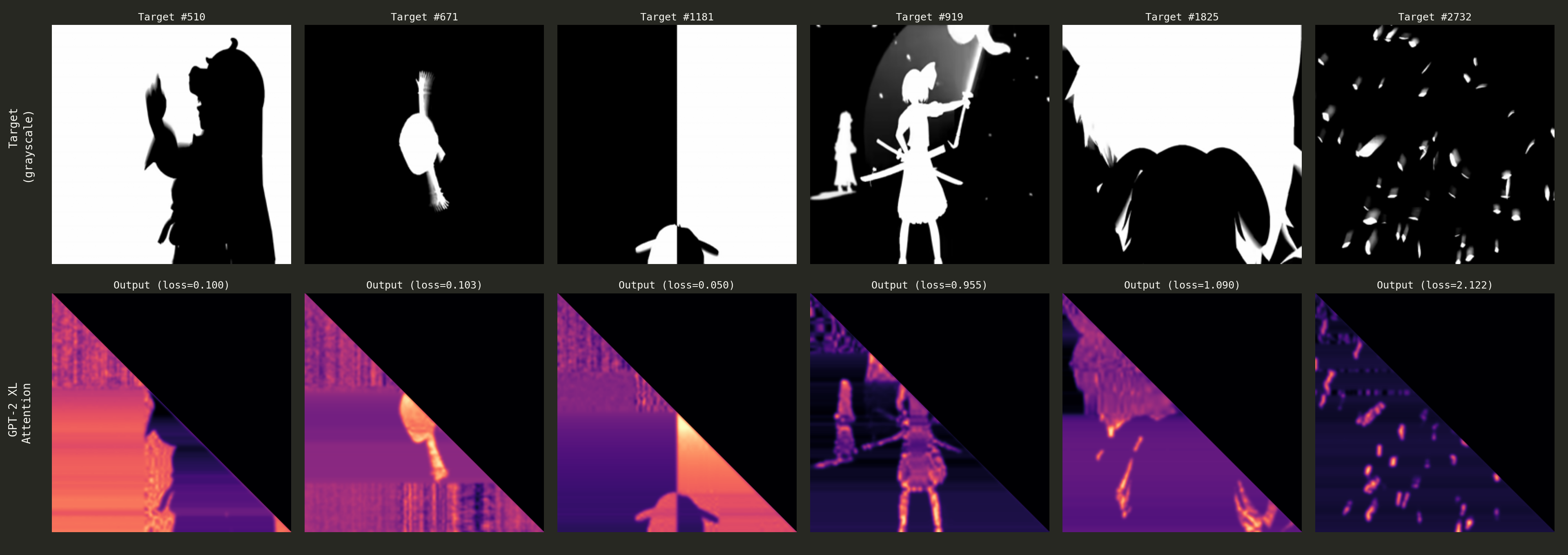Side-by-side comparison of target frames (top) and their attention map reconstructions (bottom).

Bold silhouettes and simple shapes come out great (loss as low as 0.001), while busy scenes with fine details struggle (loss up to 2.12). This makes sense: the product $QK^T$ has rank at most 64 ($d_{\text{head}}$), so it physically can’t represent arbitrary 256×256 matrices. Simple high-contrast targets fit within this rank budget, complex ones exceed it.

It’s funny to check how the loss changes across the video, you can clearly spot the different scene changes and what kind of scenes they are:

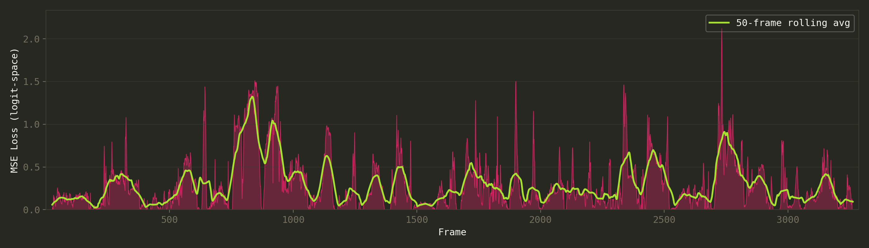Per-frame loss across the video. Spikes correspond to detailed scenes, valleys to simple silhouettes. The first ~100 frames are all-black (intro) and trivially easy.

The loss distribution is heavily right-skewed: about 81% of frames land below 0.5, 95% below 1.0, and only ~5% (152 frames) exceed 1.0. The mean loss is 0.29, median 0.18.

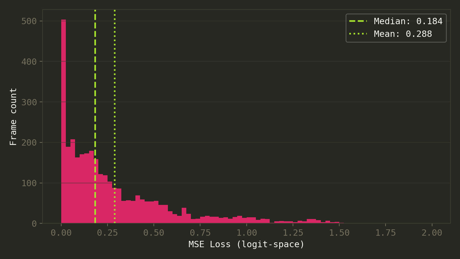Distribution of per-frame losses. Most frames cluster at low loss values, with a long tail of hard frames.

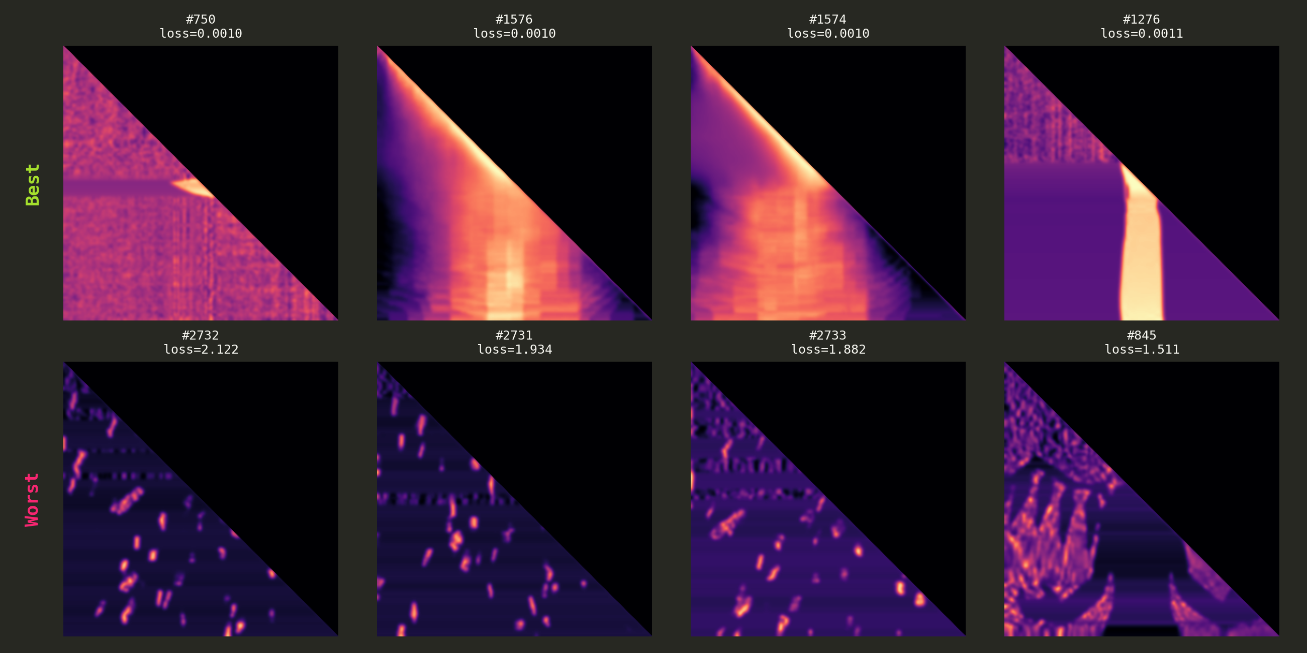Best and worst reconstructions. The optimizer nails high-contrast silhouettes but struggles with intricate details.

Note that attention maps are probability distributions (always positive, sum to 1 per row), so you can never get true black or true white in the raw output. High-contrast source material like Bad Apple’s black-and-white silhouettes works best. Subtle gradients or photographs would struggle. This approach generalizes to any high-contrast grayscale video though, not just Bad Apple.

The causal mask problem

The obvious thing visible in the resulting video is the black triangle in the top-right corner of every frame. GPT-2 is autoregressive: token $i$ can only attend to tokens $0$ through $i$, never future tokens. The upper triangle of the attention matrix is always masked (set to $-\infty$ before softmax), leaving a permanent black triangle. We lose half of the video but I found Bad Apple is still recognizable enough. Tried to mirror the bottom half to the top half but it just looked bad.

Few ideas to fix this issue:

• render each frame twice (original + transposed target), stitch the upper triangle from one and the lower from the other. Doubles compute, not really worth it for a meme project
• use a non-causal model like BERT where the full 256×256 matrix is available
• put the video in just the bottom-left quarter of the matrix

Maybe for future work!

Conclusion

I extracted the attention maps of an LLM to display the Bad Apple music video, making my own version of the meme by playing the video on another unusual “display”! To that end I used the GPT-2 XL model and optimized the input embeddings such that the attention matrix of head 0 of layer 0 matches the target frames extracted from the Bad Apple mv.

A few takeaways:

• don’t overconstrain the optimizer: single-head targeting gives it room to breathe
• avoid backpropagating through softmax when you can: logit-space loss made the difference between a stuck optimizer and a working one
• sometimes the simplest approach (one head, one frame, direct optimization) beats clever schemes

I only explored head 0 of layer 0 here, but GPT-2 XL has $25 \times 48 = 1200$ attention heads. Do some heads produce better results? Do deeper layers capture different features? Could I use 3 heads for RGB color? Material for a follow-up post.

You can find the code on GitHub. Feel free to go through it and mess with it and explore the ideas I mentioned above or render your own videos!

References

Martí, R. (2003). Multi-Start Methods. In: Handbook of Metaheuristics. Springer. https://link.springer.com/chapter/10.1007/0-306-48056-5_12 ↩︎