Understanding ComfyUI's Beta Noise Schedule

I spent some time digging into ComfyUI’s beta noise scheduling implementation and wanted to document what I found. The implementation is based on a paper from July 2024 called “Beta Sampling is All You Need”¹, which proposes using beta distribution to sample timesteps during diffusion instead of uniform sampling.

The basic idea

The core insight from the paper is pretty straightforward. When you run a diffusion model, not all timesteps contribute equally to the final image. Through Fourier analysis, the authors found that:

• Early steps handle low-frequency content (overall structure, composition)
• Late steps handle high-frequency details (edges, fine textures)
• Middle steps contribute less to perceptual quality

Traditional uniform sampling treats all timesteps equally, wasting compute on steps that don’t matter as much. Beta sampling concentrates more steps where they actually make a difference.

How ComfyUI implements it

The BetaSamplingScheduler node takes these inputs:

• model: your diffusion model
• steps: total number of sampling steps (default 20, range 1-10000)
• alpha: first beta distribution parameter (default 0.6, range 0-50)
• beta: second beta distribution parameter (default 0.6, range 0-50)

The implementation works like this:

1. Generate steps uniformly spaced values from 0 to 1
2. Pass each value through the beta distribution’s CDF
3. Scale the results to the model’s timestep range (0-999 for most SD models)
4. Convert timesteps to sigma values using the model’s noise schedule

The math looks like:

where $\text{Beta}_{\text{CDF}}(x; \alpha, \beta)$ is the cumulative distribution function of the beta distribution with parameters $\alpha$ and $\beta$.

What alpha and beta actually do

The alpha and beta parameters control the shape of the distribution:

• $\alpha = \beta$: symmetric distribution
  • Low values (< 1): concentrates samples at both ends (U-shaped)
  • Values around 1: approximately uniform
  • High values (> 1): concentrates samples in the middle (bell-shaped)
• $\alpha \neq \beta$: asymmetric distribution
  • $\alpha < \beta$: skews toward early timesteps (more denoising)
  • $\alpha > \beta$: skews toward late timesteps (more detail refinement)

The default values (0.6, 0.6) create a U-shaped distribution, putting more samples at high and low noise levels where the model’s decisions matter most.

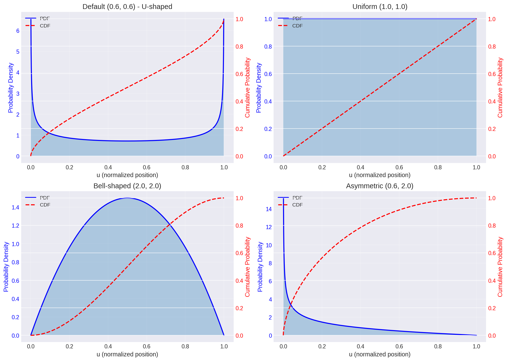Figure 1: Beta distribution PDF (solid) and CDF (dashed) for different parameter combinations. The CDF determines how timesteps are sampled.

Using it with KSamplerAdvanced

The beta scheduler outputs a sigma schedule that you feed into a sampler. With KSamplerAdvanced, you control which portion of the schedule to use via start_at_step and end_at_step.

This is different from the denoise parameter in basic KSampler. With beta scheduling:

If you use steps=20, start_at_step=0, end_at_step=20, you get full denoising. But if you use start_at_step=5, end_at_step=20, you only denoise through the portion of the schedule corresponding to those steps.

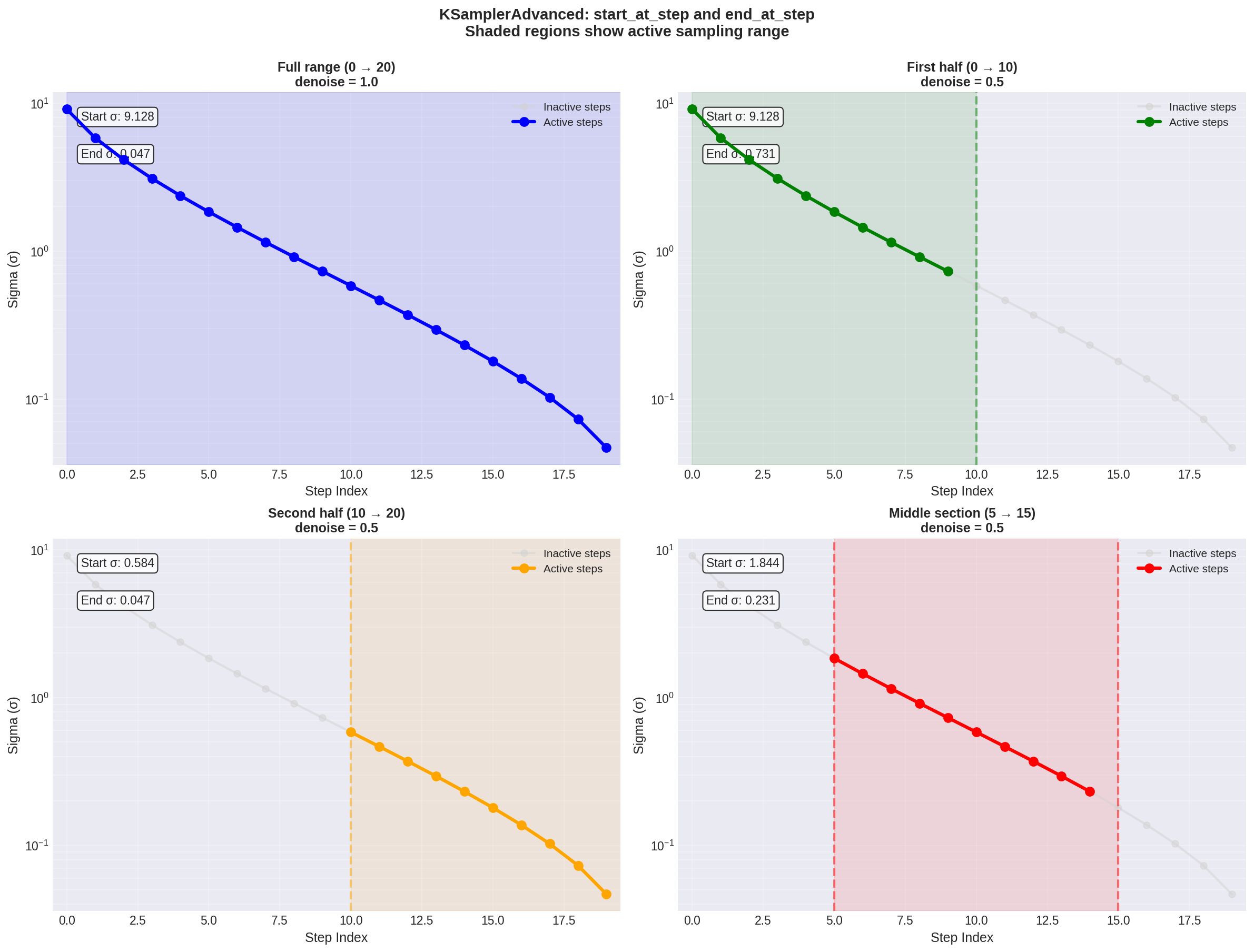Figure 2: How start_at_step and end_at_step control which portion of the sigma schedule is used. Gray dots are inactive, colored dots are active. Note how different ranges cover different noise levels.

The sigma values aren’t linearly spaced with beta sampling, so the relationship between step indices and actual noise levels is nonlinear. This is the whole point - you want more granularity where it matters.

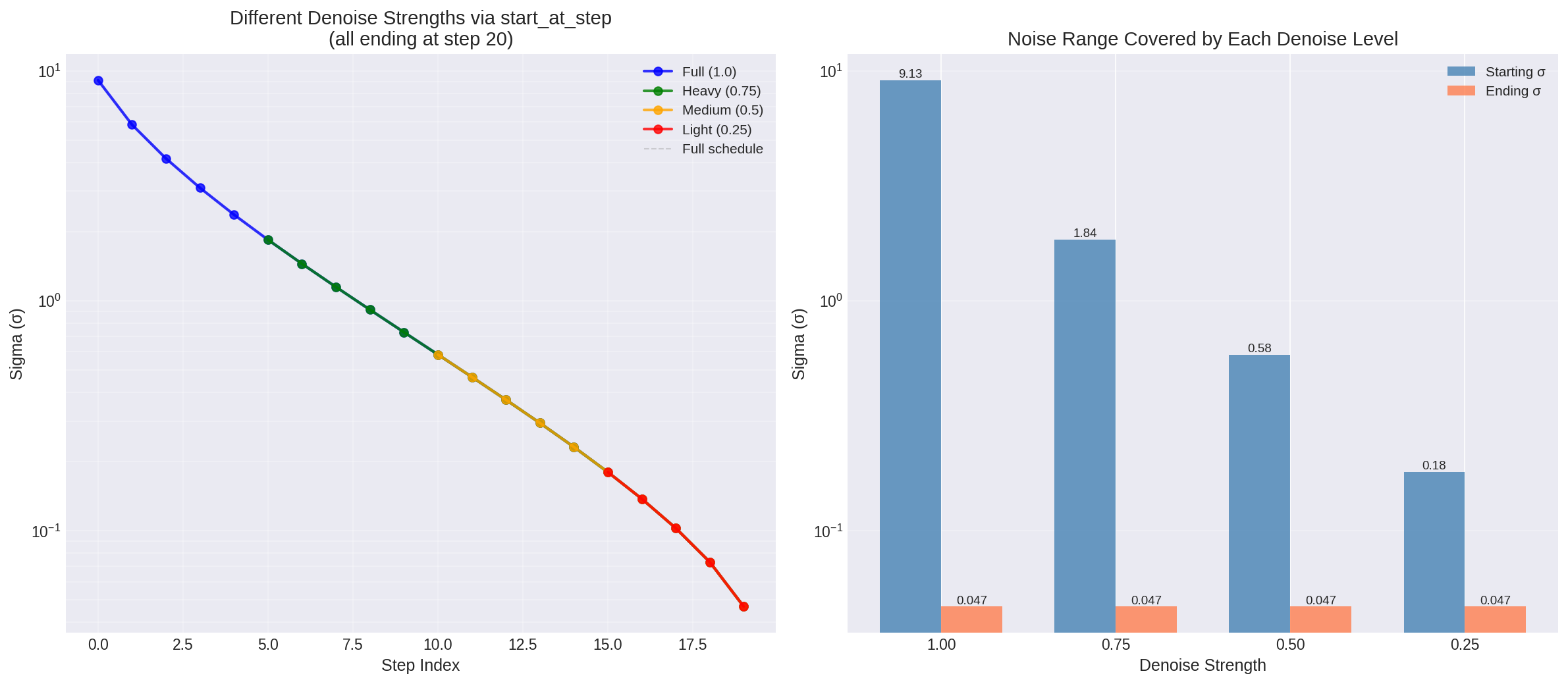Figure 3: Left - different denoise strengths achieved by varying start_at_step. Right - the actual sigma range covered by each denoise level. Lower denoise values skip the high-noise steps and start from partially denoised latents.

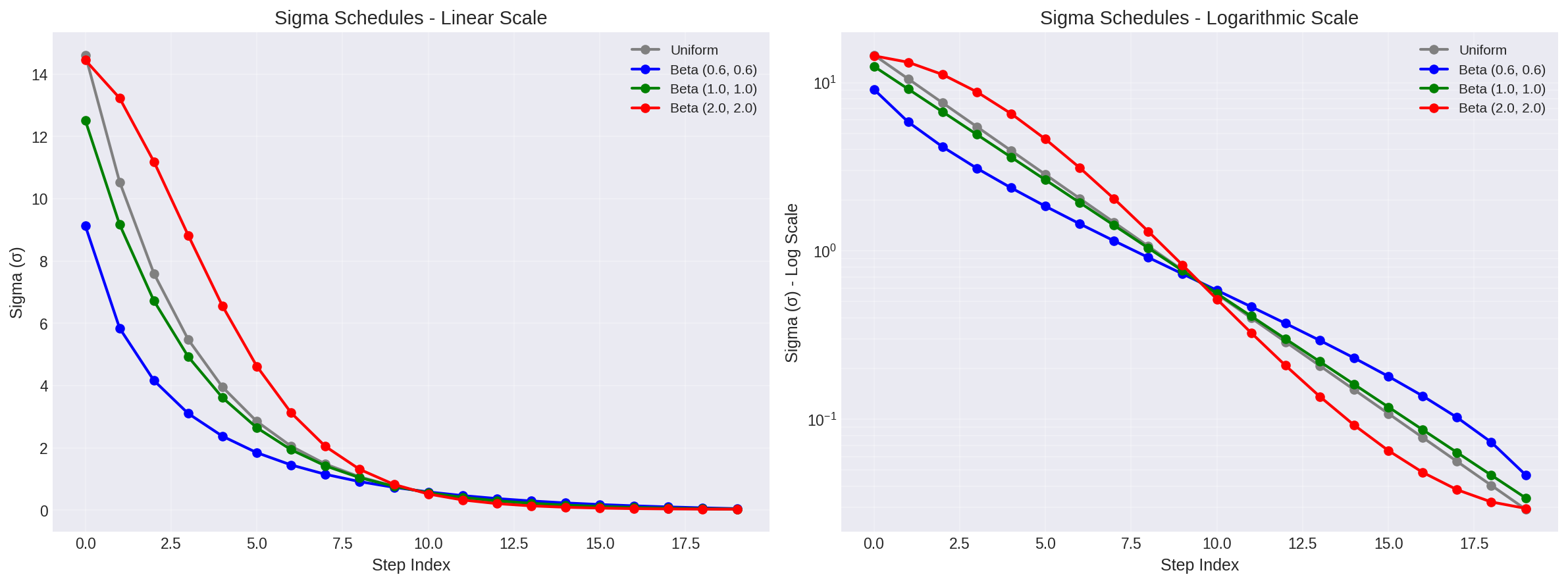Figure 4: Comparison of sigma schedules. Beta (0.6, 0.6) concentrates steps at high and low noise levels. The logarithmic scale (right) shows this more clearly.

Split sampling workflows

One of the more interesting applications of KSamplerAdvanced’s start/end step control is what I call “split sampling” and it consists of chaining multiple sampling passes with different configurations across different portions of the sigma schedule.

MoE models: the Wan2.2 case

Wan2.2’s A14B models use a Mixture-of-Experts architecture with two separate expert models trained for different noise ranges². The high-noise expert handles early denoising steps (layout and composition), while the low-noise expert refines details in later steps. Each expert is about 14B parameters, giving you 27B total capacity but only 14B active per step.

The critical part is that these experts are designed to be switched at specific timesteps. For the T2V model, you switch around timestep 0.875. For I2V, it’s around 0.900³. Note that in practice though, some people found that using a single of these two models can work well enough if you are willing to save time by avoiding loading a new model.

In ComfyUI, this means:

1. First KSamplerAdvanced: steps 0 → switch point, using high-noise expert
2. Second KSamplerAdvanced: switch point → end, using low-noise expert
3. Both share the same latent, sigma schedule, and seed

The beta scheduler becomes particularly relevant here because it naturally concentrates steps at the high and low noise extremes where the experts are most effective.

Conditional LoRA application

Another common use case is applying LoRAs only during specific diffusion stages. Say you have a style LoRA that works well for composition but mangles fine details. You can:

1. First pass (steps 0 → 10): base model only, establish layout
2. Second pass (steps 10 → 20): apply style LoRA, refine appearance

Or the reverse - use a detail-enhancement LoRA only in the final denoising steps while keeping the base model’s composition abilities for the early stages.

This is more nuanced than just adjusting LoRA strength, and reasemble more the “stop at” setting used with ContolNets. You’re selectively enabling certain model behaviors at the exact diffusion stages where they’re most useful. It’s the difference between “make this influence weaker overall” and “only use this influence during detail refinement.”

Advanced tools: ClownsharkBatwing’s approach

The RES4LYF node suite takes split sampling further with what it calls “chainsamplers”⁴. These let you chain multiple sampling passes with different:

• Samplers (e.g., RES_2M for composition, RES_5S for details)
• CFG scales
• Conditioning (you can change prompts mid-sampling)
• Noise schedules

It also includes temporal prompting for video models, where you can change conditioning on a frame-by-frame basis. The suite supports regional prompting with unlimited zones and masking, letting you apply different sampling strategies to different parts of the image simultaneously.

The key insight is that diffusion sampling doesn’t have to be monolithic. Different stages of the process benefit from different approaches, and split sampling lets you optimize each stage independently.

When to use beta scheduling

Based on the paper’s results and my own testing:

Use beta scheduling when:

• You’re doing fewer than 25 steps and want better quality
• You need fine control over early vs late sampling behavior
• You’re trying to optimize generation speed without losing quality

Stick with other schedulers when:

• You’re doing 50+ steps (diminishing returns)
• You’re using specialized sampling methods that expect uniform timesteps

Practical notes

The beta schedule can be sensitive to the model’s native noise schedule. Models trained with different noise schedules (linear, cosine, etc.) may respond differently to the same alpha/beta values.

Start with the defaults (0.6, 0.6) and adjust:

• Increase both values to concentrate samples in middle timesteps
• Decrease both to emphasize endpoints
• Make them unequal to bias toward early or late stages (e.g. bias for late stages when doing hyperrealism and towards early stages for simpler art styles)

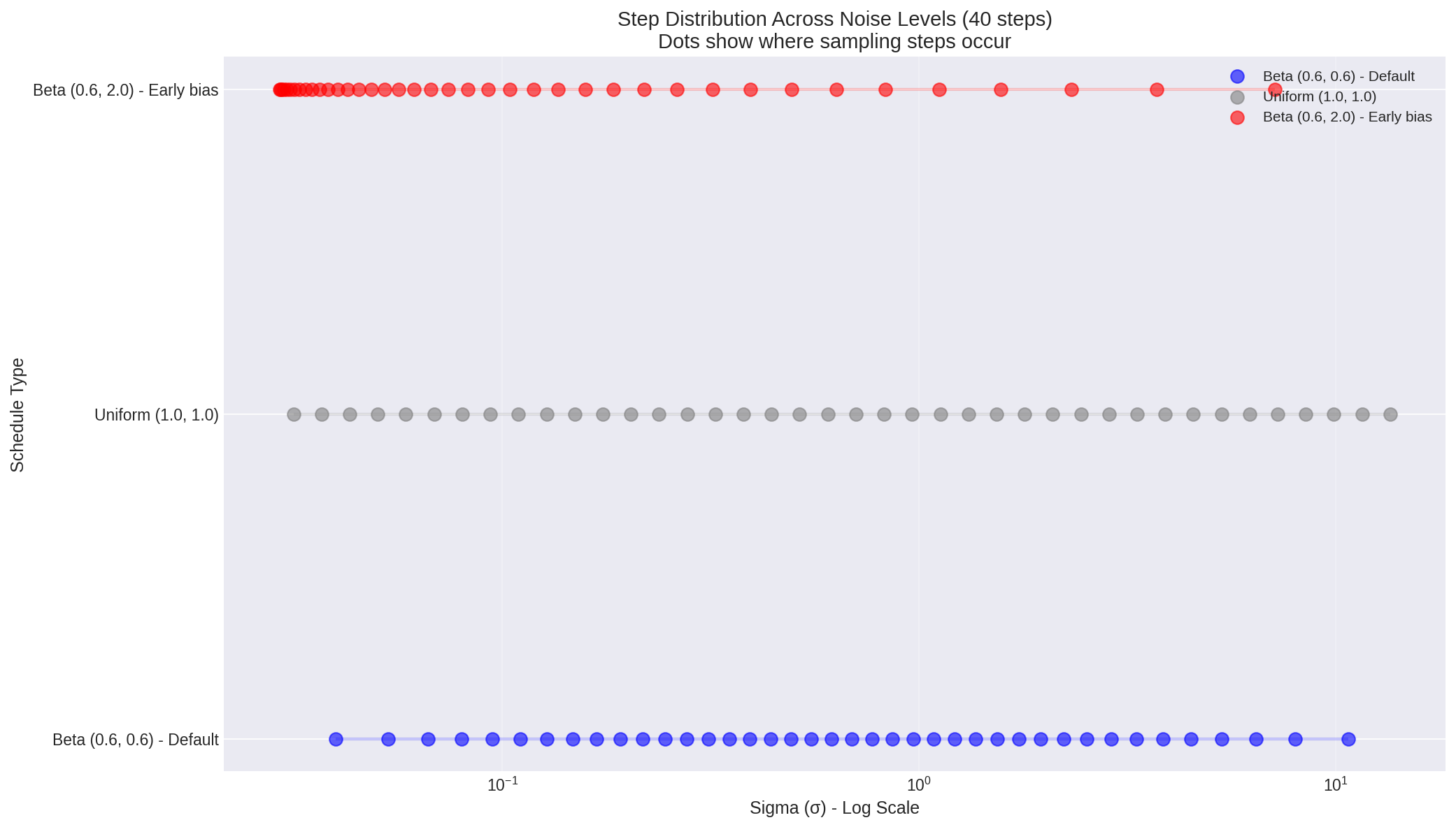Figure 5: Where sampling steps concentrate on the noise scale. Each dot represents a step. Beta (0.6, 0.6) clusters steps at the extremes, while uniform spacing is… uniform.

The math behind it

For completeness, here’s what’s actually happening under the hood. The beta distribution PDF is:

where $B(\alpha, \beta)$ is the beta function. The CDF is:

where $I_x$ is the regularized incomplete beta function.

In diffusion models, sigma represents the noise level, related to the SNR (signal-to-noise ratio) by:

where $\bar{\alpha}_t$ is the cumulative product of alphas up to timestep $t$.

The beta scheduler manipulates how we traverse this noise schedule, spending more “sampling budget” on regions of the schedule that contribute most to image quality.

Implementation details

ComfyUI’s actual implementation is in comfy_extras/nodes_custom_sampler.py. The node is simple - it’s essentially a wrapper around scipy’s beta distribution CDF, mapping the output to model timesteps and converting those to sigmas.

The interesting part is how it interacts with the rest of the sampling pipeline. The sigma schedule it produces is just a sequence of noise levels. The actual sampler (Euler, DPM++, etc.) handles how to step through that schedule.

You can think of it like this:

• Beta scheduler: “Here’s where we should sample”
• Sampler: “Here’s how we should sample”
• Model: “Here’s what we should predict”

They’re orthogonal concerns, which is why you can mix and match schedulers with samplers freely.

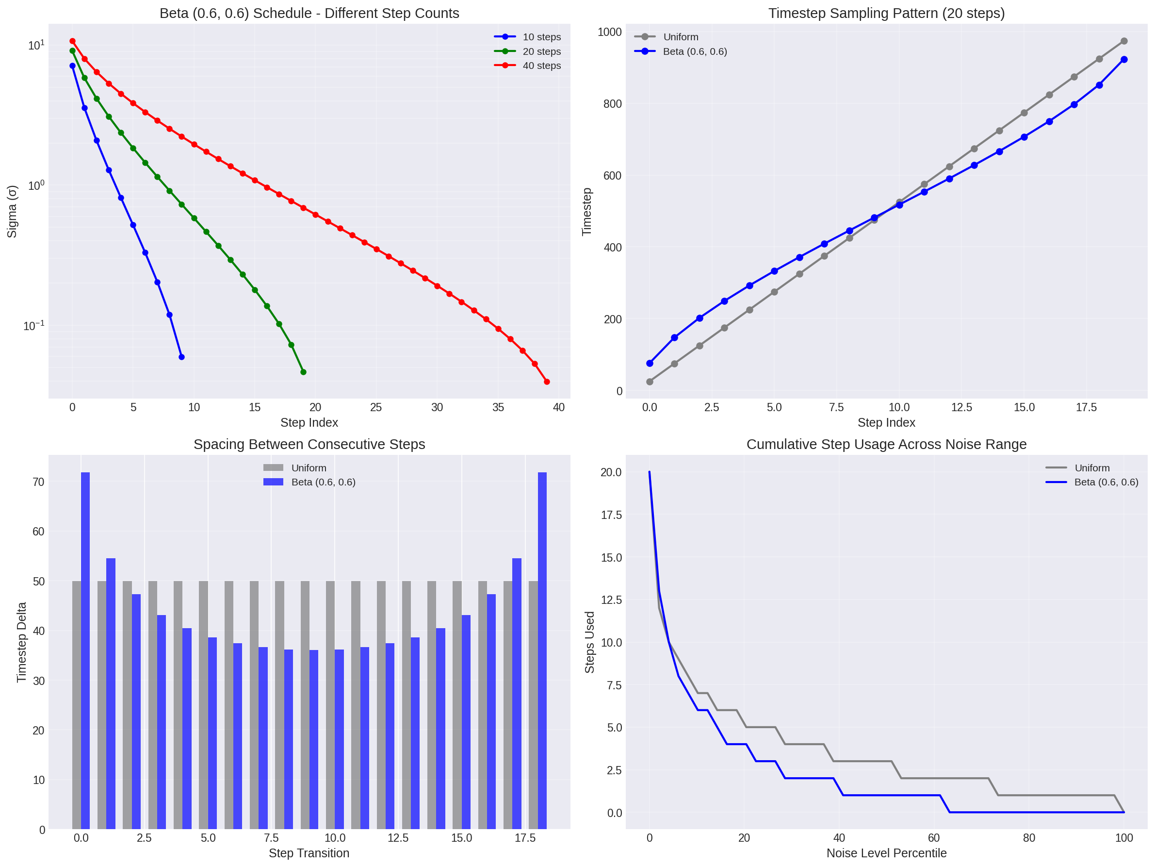Figure 6: Detailed behavior of beta scheduling. Top left: how it scales with step count. Top right: timestep sampling pattern. Bottom left: spacing between steps (note the U-shape). Bottom right: cumulative step usage shows beta scheduling front-loads and back-loads the sampling budget.

Conclusion

The beta noise scheduler represents a meaningful improvement over uniform timestep sampling for diffusion models. By concentrating sampling steps at the noise levels where models make the most significant perceptual decisions, it achieves better image quality with fewer steps. The paper’s spectral analysis provides solid empirical justification for this approach, and the implementation in ComfyUI makes it accessible for practical use.

The scheduler’s flexibility through alpha and beta parameters allows fine-tuning for different use cases, from aggressive low-step generation to specialized workflows like split sampling for MoE models. Its non-uniform distribution is particularly valuable when working with models that have distinct behavior patterns across different noise levels.

The mathematical foundation is straightforward - using the beta distribution’s CDF to map uniform samples to timesteps - but the practical implications are significant. Combined with advanced sampling techniques and proper parameter tuning, beta scheduling can noticeably improve results compared to traditional schedulers at similar step counts.

For practical work, I’ve found it’s my favorite schedule when paired with the Euler sampler for realism with Flux.1 [dev], especially when biasing slighly towards late stages for improved details ($\alpha=1.0$, $\beta=0.6$ works fine, adjust if needed, experimentationn is key!).

References

Lee, H., Lee, H., Gye, S., & Kim, J. (2024). Beta Sampling is All You Need: Efficient Image Generation Strategy for Diffusion Models using Stepwise Spectral Analysis. arXiv:2407.12173. https://arxiv.org/abs/2407.12173 ↩︎
Wan-Video. (2024). Wan2.2: Open and Advanced Large-Scale Video Generative Models. https://github.com/Wan-Video/Wan2.2 ↩︎
stduhpf. (2024). ComfyUI-WanMoeKSampler. https://github.com/stduhpf/ComfyUI-WanMoeKSampler ↩︎
ClownsharkBatwing. (2024). RES4LYF: Advanced Sampling Suite for ComfyUI. https://github.com/ClownsharkBatwing/RES4LYF ↩︎